Usage of the Landweber class

We illustrate the usage and available methods of the Landweber class via a small example.

import numpy as np
import matplotlib.pyplot as plt
import EarlyStopping as es
from scipy.sparse import dia_matrix
import seaborn as sns

np.random.seed(42)
sns.set_theme()

Generating synthetic data

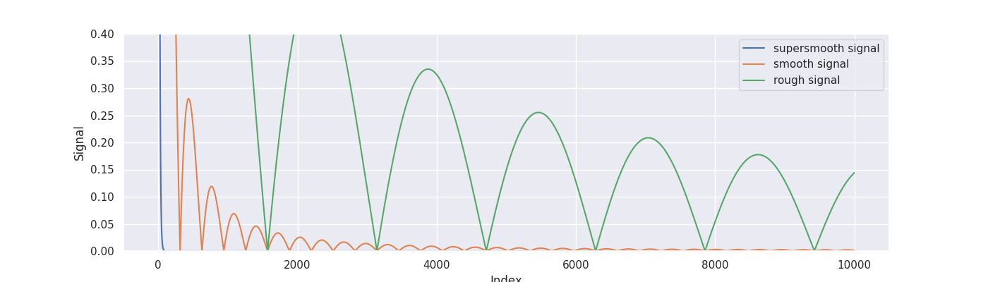
To simulate some data we consider the signals from Blanchard, Hoffmann and Reiß (2018).

sample_size = 10000
indices = np.arange(sample_size) + 1

signal_supersmooth = 5 * np.exp(-0.1 * indices)
signal_smooth = 5000 * np.abs(np.sin(0.01 * indices)) * indices ** (-1.6)
signal_rough = 250 * np.abs(np.sin(0.002 * indices)) * indices ** (-0.8)

true_signal = signal_rough

plt.figure(figsize=(14, 4))
plt.plot(indices, signal_supersmooth, label="supersmooth signal")
plt.plot(indices, signal_smooth, label="smooth signal")
plt.plot(indices, signal_rough, label="rough signal")
plt.ylabel("Signal")
plt.xlabel("Index")
plt.ylim([0, 0.4])
plt.legend(loc="upper right")
plt.show()

We simulate data from a prototypical inverse problem based on one of the signals

true_noise_level = 0.01
noise = true_noise_level * np.random.normal(0, 1, sample_size)

eigenvalues = 1 / np.sqrt(indices)
design = dia_matrix(np.diag(eigenvalues))

response = eigenvalues * true_signal + noise

# Initialize Landweber class
alg = es.Landweber(design, response, learning_rate=1, true_signal=true_signal, true_noise_level=true_noise_level)
alg.iterate(3000)

UserWarning: No initial_value is given, using zero by default.
SparseEfficiencyWarning: spsolve requires A be CSC or CSR matrix format
SparseEfficiencyWarning: spsolve is more efficient when sparse b is in the CSC matrix format

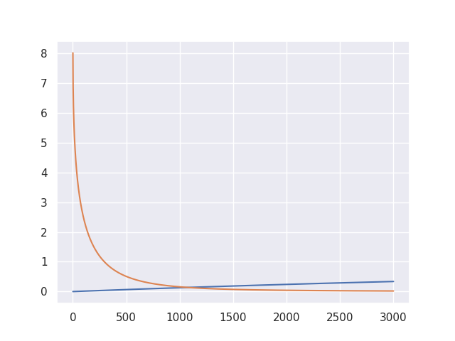
Bias-variance decomposition (weak/strong)

plt.figure()
plt.plot(indices[0 : alg.iteration + 1], alg.weak_variance, label="Weak variance")
plt.plot(indices[0 : alg.iteration + 1], alg.weak_bias2, label="Weak squared bias")
plt.legend(loc="upper right")
plt.show()

plt.figure()
plt.plot(indices[0 : alg.iteration + 1], alg.strong_variance, label="Strong variance")
plt.plot(indices[0 : alg.iteration + 1], alg.strong_bias2, label="Strong squared bias")
plt.legend(loc="upper right")
plt.show()

print(f"Weak balanced oracle: {alg.get_weak_balanced_oracle(3000)}")
print(f"Strong balanced oracle: {alg.get_strong_balanced_oracle(3000)}")

• 
• 

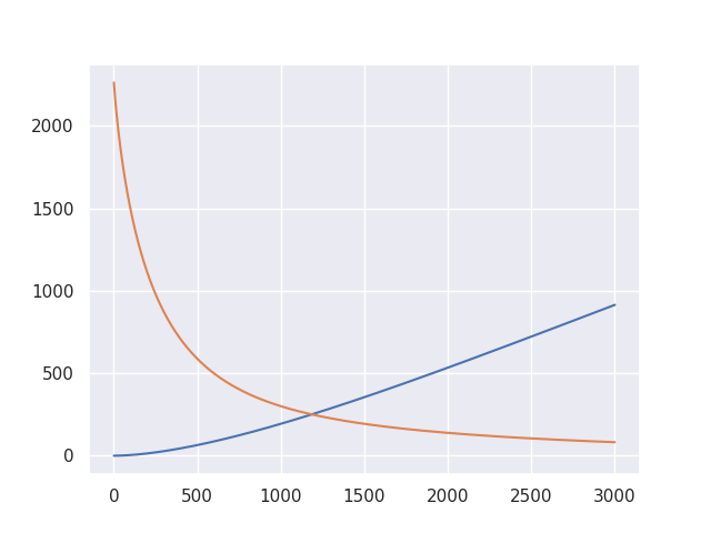
Weak balanced oracle: 1074
Strong balanced oracle: 1185

Early stopping w/ discrepancy principle

critical_value = sample_size * true_noise_level**2
discrepancy_time = alg.get_discrepancy_stop(critical_value, 3000)
estimated_signal = alg.get_estimate(discrepancy_time)

print(f"Critical value: {critical_value}.")
print(f"Discrepancy stopping time: {discrepancy_time}")

plt.figure(figsize=(14, 4))
plt.plot(indices, estimated_signal, label="Estimated signal at stopping time")
plt.plot(indices, true_signal, label="True signal")
plt.ylim([0, 2])
plt.legend(loc="upper right")
plt.show()

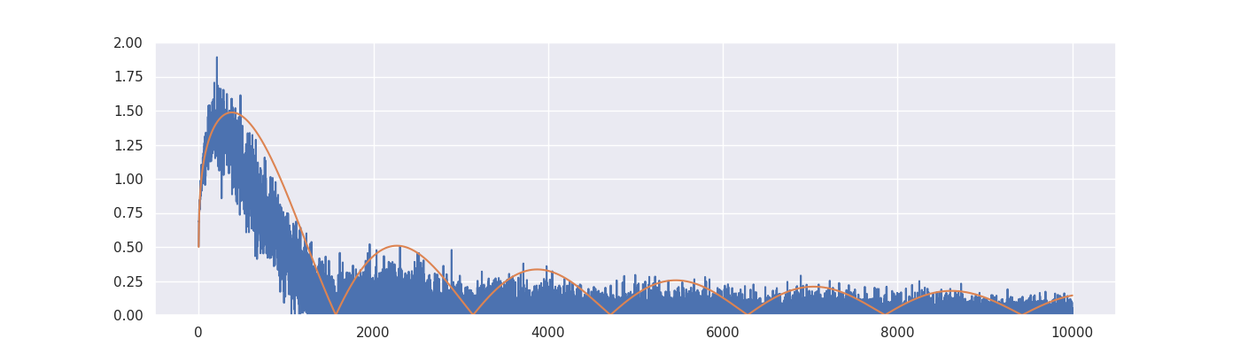
Critical value: 1.0.
Discrepancy stopping time: 670