Usage of the L2-boost class

We illustrate the available methods of the L2-boost class via a small example.

import numpy as np
import matplotlib.pyplot as plt
import seaborn as sns
import EarlyStopping as es

np.random.seed(42)
sns.set_theme()

Generating synthetic data

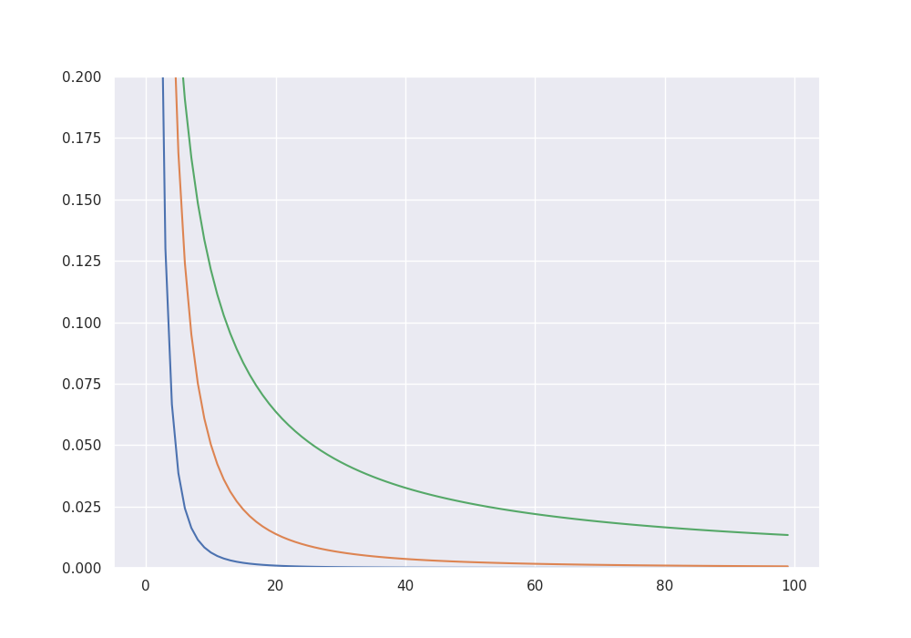
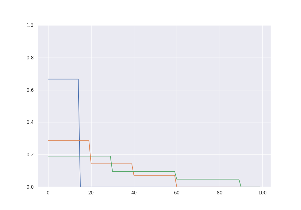
To simulate some data we consider the signals from Stankewitz (2022).

sample_size = 1000
para_size = 1000

# Gamma-sparse signals
beta_3 = 1 / (1 + np.arange(para_size)) ** 3
beta_3 = 10 * beta_3 / np.sum(np.abs(beta_3))

beta_2 = 1 / (1 + np.arange(para_size)) ** 2
beta_2 = 10 * beta_2 / np.sum(np.abs(beta_2))

beta_1 = 1 / (1 + np.arange(para_size))
beta_1 = 10 * beta_1 / np.sum(np.abs(beta_1))

# S-sparse signals
beta_15 = np.zeros(para_size)
beta_15[0:15] = 1
# beta_15[10:15] = 0.1
beta_15 = 10 * beta_15 / np.sum(np.abs(beta_15))

beta_60 = np.zeros(para_size)
beta_60[0:20] = 1
beta_60[20:40] = 0.5
beta_60[40:60] = 0.25
beta_60 = 10 * beta_60 / np.sum(np.abs(beta_60))

beta_90 = np.zeros(para_size)
beta_90[0:30] = 1
beta_90[30:60] = 0.5
beta_90[60:90] = 0.25
beta_90 = 10 * beta_90 / np.sum(np.abs(beta_90))

fig = plt.figure(figsize=(10, 7))
plt.ylim(0, 0.2)
plt.plot(beta_3[0:100])
plt.plot(beta_2[0:100])
plt.plot(beta_1[0:100])
plt.show()

fig = plt.figure(figsize=(10, 7))
plt.ylim(0, 1)
plt.plot(beta_15[0:100])
plt.plot(beta_60[0:100])
plt.plot(beta_90[0:100])
plt.show()

• 
• 

We simulate data from a high-dimensional linear model according to one of the signals.

cov = np.identity(para_size)
sigma = np.sqrt(1)
X = np.random.multivariate_normal(np.zeros(para_size), cov, sample_size)
f = X @ beta_15
eps = np.random.normal(0, sigma, sample_size)
Y = f + eps

Theoretical bias-variance decomposition

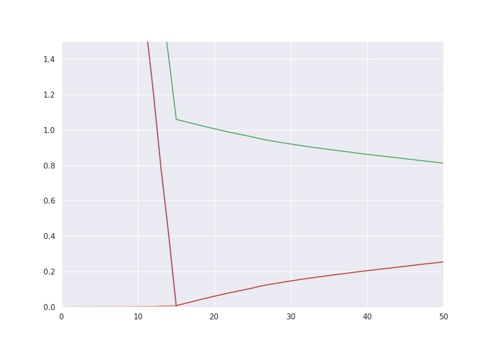
By giving the true function f to the class, we can track the theoretical bias-variance decomposition and the balanced oracle.

alg = es.L2_boost(X, Y, beta_15)
alg.get_balanced_oracle(20)
print("The balanced oracle is given by", alg.iteration, "with risk =", alg.risk[alg.iteration])
alg.iterate(50 - alg.iteration)
classical_oracle = np.argmin(alg.risk)
print("The classical oracle is given by", classical_oracle, "with risk =", alg.risk[classical_oracle])

fig = plt.figure(figsize=(10, 7))
plt.plot(alg.bias2)
plt.plot(alg.stochastic_error)
plt.plot(alg.residuals)
plt.plot(alg.risk)
plt.ylim((0, 1.5))
plt.xlim((0, 50))
plt.show()

The balanced oracle is given by 15 with risk = 0.007929012522306171
The classical oracle is given by 15 with risk = 0.007929012522306171

Early stopping via the discrepancy principle

The L2-boost class provides several data driven methods to choose a boosting iteration making the right tradeoff between bias and stochastic error. The first one is a stopping condition based on the discrepancy principle, which stops when the residuals become smaller than a critical value. Theoretically this critical value should be chosen as the noise level of the model, for which the class also provides a methods based on the scaled Lasso.

noise_estimate = alg.get_noise_estimate(K = 0.5)
stopping_time = alg.get_discrepancy_stop(critical_value = noise_estimate, max_iteration=200)
stopping_time
print("The discrepancy based early stopping time is given by", stopping_time, "with risk =",
      alg.risk[stopping_time])

np.sqrt(np.min(alg.risk) / alg.risk[stopping_time])
alg.risk

The discrepancy based early stopping time is given by 27 with risk = 0.1261508860716641

array([6.52912946, 5.92477128, 5.34282147, 4.83987233, 4.34696072,
       3.89008948, 3.39245076, 3.03832344, 2.67500904, 2.33798263,
       1.94839193, 1.5996138 , 1.21572015, 0.78919039, 0.41534997,
       0.00792901, 0.01902339, 0.02961507, 0.04066919, 0.05085466,
       0.06135702, 0.07098903, 0.08061858, 0.089467  , 0.09842829,
       0.10748952, 0.11780136, 0.12615089, 0.13331796, 0.1406172 ,
       0.14717897, 0.15406691, 0.16046815, 0.16643022, 0.17229239,
       0.17816578, 0.18362908, 0.1888606 , 0.19450746, 0.20049679,
       0.20557095, 0.21038042, 0.2155474 , 0.22050148, 0.22543476,
       0.23040747, 0.23555005, 0.24068679, 0.24528587, 0.25009712,
       0.25529961])

Early stopping via residual ratios

Another method is based on stopping when the ratio of consecutive residuals goes above a certain threshhold.

stopping_time = alg.get_residual_ratio_stop(max_iteration=200, K=1.2)
print("The residual ratio based early stopping time is given by", stopping_time, "with risk =",
      alg.risk[stopping_time])

stopping_time = alg.get_residual_ratio_stop(max_iteration=200, K=0.2)
print("The residual ratio based early stopping time is given by", stopping_time, "with risk =",
      alg.risk[stopping_time])

stopping_time = alg.get_residual_ratio_stop(max_iteration=200, K=0.1)
print("The residual ratio based early stopping time is given by", stopping_time, "with risk =",
      alg.risk[stopping_time])

The residual ratio based early stopping time is given by 16 with risk = 0.01902338799162816
The residual ratio based early stopping time is given by 28 with risk = 0.13331795792320866
The residual ratio based early stopping time is given by 143 with risk = 0.5606822045222807

Classical model selection via AIC

The class also has a method to compute a high dimensional Akaike criterion over the boosting path up to the current iteration.

aic_minimizer = alg.get_aic_iteration(K=2)
print("The aic-minimizer over the whole path is given by", aic_minimizer, "with risk =", alg.risk[aic_minimizer])

The aic-minimizer over the whole path is given by 15 with risk = 0.007929012522306171