Note
Go to the end to download the full example code.
This is a simulation example of the Landweber class.#
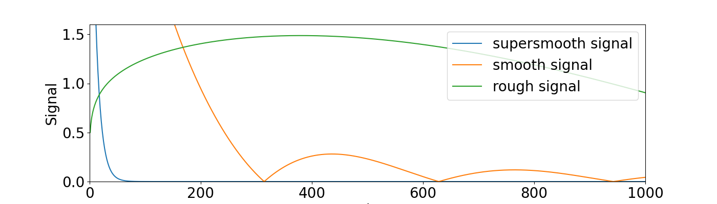
It is based on the generated supersmooth, smooth and rough signal of Blanchard et al. (2018).
import matplotlib.pyplot as plt
import numpy as np
import EarlyStopping as es
from scipy.sparse import dia_matrix
import timeit

np.random.seed(42)
plt.rcParams.update({"font.size": 20})
print('The seed is 42.')
The seed is 42.
Plot different signals#
Create diagonal design matrix and supersmooth, smooth and rough signal. Plot the signal.
D = 10000
indices = np.arange(D) + 1
design_matrix = dia_matrix(np.diag(1 / (np.sqrt(indices))))

signal_supersmooth = 5 * np.exp(-0.1 * indices)
signal_smooth = 5000 * np.abs(np.sin(0.01 * indices)) * indices ** (-1.6)
signal_rough = 250 * np.abs(np.sin(0.002 * indices)) * indices ** (-0.8)

plt.figure(figsize=(14, 4))
plt.plot(indices, signal_supersmooth, label="supersmooth signal")
plt.plot(indices, signal_smooth, label="smooth signal")
plt.plot(indices, signal_rough, label="rough signal")
plt.ylabel("Signal")
plt.xlabel("Index")
plt.xlim([0, 1000])
plt.ylim([0, 1.6])
plt.legend(loc="upper right")
plt.show()
Generate data and run Landweber#
Run the Landweber algorithm and get the early stopping index as well as as the weak/strong balanced oracle.
NOISE_LEVEL = 0.01
noise = np.random.normal(0, NOISE_LEVEL, D)

observation_supersmooth = noise + design_matrix @ signal_supersmooth
observation_smooth = noise + design_matrix @ signal_smooth
observation_rough = noise + design_matrix @ signal_rough


models_supersmooth = es.Landweber(design_matrix, observation_supersmooth, true_signal=signal_supersmooth, learning_rate=1,
                                  true_noise_level=NOISE_LEVEL)
models_smooth = es.Landweber(design_matrix, observation_smooth, true_signal=signal_smooth, learning_rate=1,
                             true_noise_level=NOISE_LEVEL)
models_rough = es.Landweber(design_matrix, observation_rough, true_signal=signal_rough, learning_rate=1,
                            true_noise_level=NOISE_LEVEL)

# models_supersmooth = es.Landweber(
#     design_matrix, observation_supersmooth, true_noise_level=NOISE_LEVEL, true_signal=signal_supersmooth
# )
# models_smooth = es.Landweber(design_matrix, observation_smooth, true_noise_level=NOISE_LEVEL, true_signal=signal_smooth)
# models_rough = es.Landweber(design_matrix, observation_rough, true_noise_level=NOISE_LEVEL, true_signal=signal_rough)

max_iteration = 1500
start = timeit.default_timer()
models_supersmooth.iterate(max_iteration)
stop = timeit.default_timer()
print("Time supersmooth: ", stop - start)

#models_supersmooth.landweber_estimate_collect

start = timeit.default_timer()
models_smooth.iterate(max_iteration)
stop = timeit.default_timer()
print("Time smooth: ", stop - start)

start = timeit.default_timer()
models_rough.iterate(max_iteration)
stop = timeit.default_timer()
print("Time rough: ", stop - start)

# Stopping index
supersmooth_m = models_supersmooth.get_discrepancy_stop(D*(NOISE_LEVEL**2), max_iteration)
smooth_m = models_smooth.get_discrepancy_stop(D*(NOISE_LEVEL**2), max_iteration)
rough_m = models_rough.get_discrepancy_stop(D*(NOISE_LEVEL**2), max_iteration)

# Weak balanced oracle
supersmooth_weak_oracle = models_supersmooth.get_weak_balanced_oracle(max_iteration)
smooth_weak_oracle = models_smooth.get_weak_balanced_oracle(max_iteration)
rough_weak_oracle = models_rough.get_weak_balanced_oracle(max_iteration)

# Strong balanced oracle
supersmooth_strong_oracle = models_supersmooth.get_strong_balanced_oracle(max_iteration)
smooth_strong_oracle = models_smooth.get_strong_balanced_oracle(max_iteration)
rough_strong_oracle = models_rough.get_strong_balanced_oracle(max_iteration)
/opt/hostedtoolcache/Python/3.12.7/x64/lib/python3.12/site-packages/EarlyStopping/landweber.py:115: UserWarning: No initial_value is given, using zero by default.
  warnings.warn("No initial_value is given, using zero by default.", category=UserWarning)
/opt/hostedtoolcache/Python/3.12.7/x64/lib/python3.12/site-packages/scipy/sparse/linalg/_dsolve/linsolve.py:603: SparseEfficiencyWarning: splu converted its input to CSC format
  return splu(A).solve
/opt/hostedtoolcache/Python/3.12.7/x64/lib/python3.12/site-packages/scipy/sparse/linalg/_matfuncs.py:76: SparseEfficiencyWarning: spsolve is more efficient when sparse b is in the CSC matrix format
  Ainv = spsolve(A, I)
Time supersmooth:  3.809562239999991
Time smooth:  3.844058907999994
Time rough:  3.8659052120000013
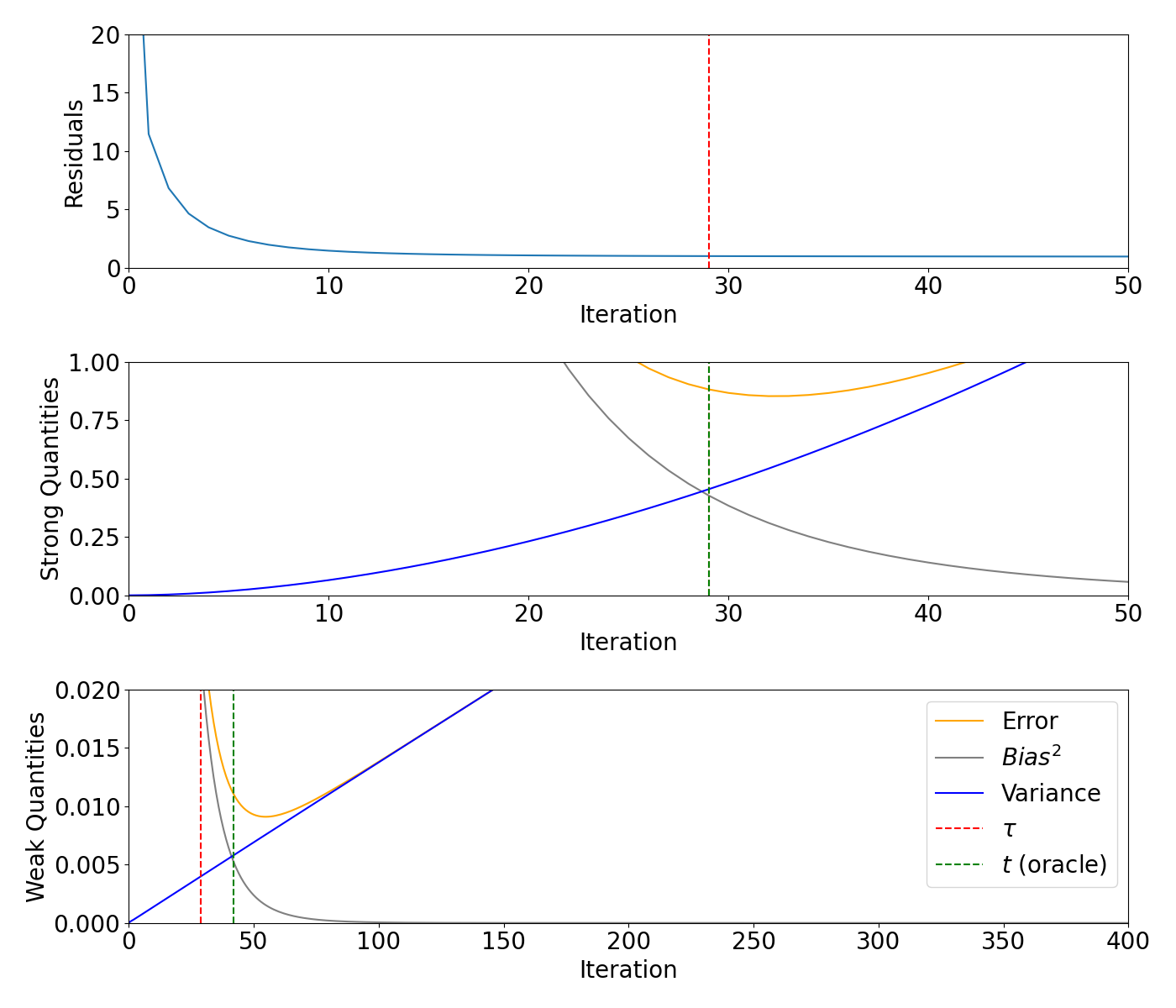
Bias/variance decomposition for supersmooth signal#
Plot the residuals, weak and strong quantities for the supersmooth signal.
# plt.rcParams.update({'font.size': 18})  # Update the font size

fig, axs = plt.subplots(3, 1, figsize=(14, 12))


axs[0].plot(range(0, max_iteration + 1), models_supersmooth.residuals)
axs[0].axvline(x=supersmooth_m, color="red", linestyle="--")
axs[0].set_xlim([0, 50])
axs[0].set_ylim([0, 20])
axs[0].set_xlabel("Iteration")
axs[0].set_ylabel("Residuals")


axs[1].plot(range(0, max_iteration + 1), models_supersmooth.strong_risk, color="orange", label="Error")
axs[1].plot(range(0, max_iteration + 1), models_supersmooth.strong_bias2, label="$Bias^2$", color="grey")
axs[1].plot(range(0, max_iteration + 1), models_supersmooth.strong_variance, label="Variance", color="blue")
axs[1].axvline(x=supersmooth_m, color="red", linestyle="--")
axs[1].axvline(x=supersmooth_strong_oracle, color="green", linestyle="--")
axs[1].set_xlim([0, 50])
axs[1].set_ylim([0, 1])
axs[1].set_xlabel("Iteration")
axs[1].set_ylabel("Strong Quantities")

axs[2].plot(range(0, max_iteration + 1), models_supersmooth.weak_risk, color="orange", label="Error")
axs[2].plot(range(0, max_iteration + 1), models_supersmooth.weak_bias2, label="$Bias^2$", color="grey")
axs[2].plot(range(0, max_iteration + 1), models_supersmooth.weak_variance, label="Variance", color="blue")
axs[2].axvline(x=supersmooth_m, color="red", linestyle="--", label=r"$\tau$")
axs[2].axvline(x=supersmooth_weak_oracle, color="green", linestyle="--", label="$t$ (oracle)")
axs[2].set_xlim([0, 400])
axs[2].set_ylim([0, 0.02])
axs[2].set_xlabel("Iteration")
axs[2].set_ylabel("Weak Quantities")
axs[2].legend()

plt.tight_layout()

plt.show()
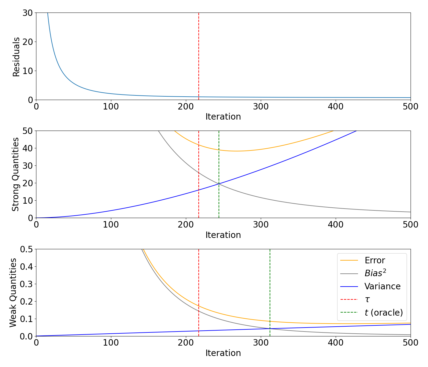
Bias/variance decomposition for smooth signal#
Plot the residuals, weak and strong quantities for the smooth signal.
fig, axs = plt.subplots(3, 1, figsize=(14, 12))

axs[0].plot(range(0, max_iteration + 1), models_smooth.residuals)
axs[0].axvline(x=smooth_m, color="red", linestyle="--")
axs[0].set_xlim([0, 500])
axs[0].set_ylim([0, 30])
axs[0].set_xlabel("Iteration")
axs[0].set_ylabel("Residuals")

axs[1].plot(range(0, max_iteration + 1), models_smooth.strong_risk, color="orange", label="Error")
axs[1].plot(range(0, max_iteration + 1), models_smooth.strong_bias2, label="$Bias^2$", color="grey")
axs[1].plot(range(0, max_iteration + 1), models_smooth.strong_variance, label="Variance", color="blue")
axs[1].axvline(x=smooth_m, color="red", linestyle="--")
axs[1].axvline(x=smooth_strong_oracle, color="green", linestyle="--")
axs[1].set_xlim([0, 500])
axs[1].set_ylim([0, 50])
axs[1].set_xlabel("Iteration")
axs[1].set_ylabel("Strong Quantities")

axs[2].plot(range(0, max_iteration + 1), models_smooth.weak_risk, color="orange", label="Error")
axs[2].plot(range(0, max_iteration + 1), models_smooth.weak_bias2, label="$Bias^2$", color="grey")
axs[2].plot(range(0, max_iteration + 1), models_smooth.weak_variance, label="Variance", color="blue")
axs[2].axvline(x=smooth_m, color="red", linestyle="--", label=r"$\tau$")
axs[2].axvline(x=smooth_weak_oracle, color="green", linestyle="--", label="$t$ (oracle)")
axs[2].set_xlim([0, 500])
axs[2].set_ylim([0, 0.5])
axs[2].set_xlabel("Iteration")
axs[2].set_ylabel("Weak Quantities")
axs[2].legend()

plt.tight_layout()

plt.show()
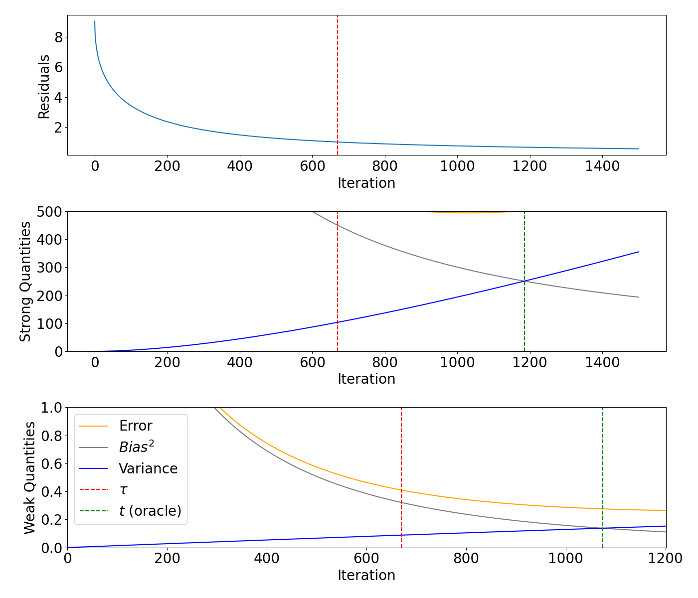
Bias/variance decomposition for rough signal#
Plot the residuals, weak and strong quantities for the rough signal.
fig, axs = plt.subplots(3, 1, figsize=(14, 12))

axs[0].plot(range(0, max_iteration + 1), models_rough.residuals)
axs[0].axvline(x=rough_m, color="red", linestyle="--")
axs[0].set_xlabel("Iteration")
axs[0].set_ylabel("Residuals")

axs[1].plot(range(0, max_iteration + 1), models_rough.strong_risk, color="orange", label="Error")
axs[1].plot(range(0, max_iteration + 1), models_rough.strong_bias2, label="$Bias^2$", color="grey")
axs[1].plot(range(0, max_iteration + 1), models_rough.strong_variance, label="Variance", color="blue")
axs[1].axvline(x=rough_m, color="red", linestyle="--")
axs[1].axvline(x=rough_strong_oracle, color="green", linestyle="--")
axs[1].set_ylim([0, 500])
axs[1].set_xlabel("Iteration")
axs[1].set_ylabel("Strong Quantities")

axs[2].plot(range(0, max_iteration + 1), models_rough.weak_risk, color="orange", label="Error")
axs[2].plot(range(0, max_iteration + 1), models_rough.weak_bias2, label="$Bias^2$", color="grey")
axs[2].plot(range(0, max_iteration + 1), models_rough.weak_variance, label="Variance", color="blue")
axs[2].axvline(x=rough_m, color="red", linestyle="--", label=r"$\tau$")
axs[2].axvline(x=rough_weak_oracle, color="green", linestyle="--", label="$t$ (oracle)")
axs[2].set_xlim([0, 1200 + 1])
axs[2].set_ylim([0, 1])
axs[2].set_xlabel("Iteration")
axs[2].set_ylabel("Weak Quantities")
axs[2].legend()

plt.tight_layout()
plt.show()
Bias/variance decomposition for the gravity example#
Gravity test problem from the regtools toolbox, see Hansen (2008) for details. Plot the residuals, weak and strong quantities.
sample_size = 100  # 2**9
a = 0
b = 1
d = 0.25  # Parameter controlling the ill-posedness: the larger, the more ill-posed, default in regtools: d = 0.25

t = (np.arange(1, sample_size + 1) - 0.5) / sample_size
s = ((np.arange(1, sample_size + 1) - 0.5) * (b - a)) / sample_size
T, S = np.meshgrid(t, s)

design = (1 / sample_size) * d * (d**2 * np.ones((sample_size, sample_size)) + (S - T) ** 2) ** (-(3 / 2))
signal = np.sin(np.pi * t) + 0.5 * np.sin(2 * np.pi * t)
design_times_signal = design @ signal

# Set parameters
parameter_size = sample_size
max_iteration = 2000
noise_level = 10 ** (-2)
# critical_value = sample_size * (noise_level**2)

#eigen_values = np.linalg.eig(design)
#print(f"The eigenvalues are given by \n {eigen_values}")

# Specify number of Monte Carlo runs
NUMBER_RUNS = 1

# Create observations
noise = np.random.normal(0, noise_level, (sample_size, NUMBER_RUNS))
observation = noise + design_times_signal[:, None]

model_gravity = es.Landweber(design, observation[:, 0], learning_rate=1 / 30, true_signal=signal, true_noise_level=noise_level)

model_gravity.iterate(max_iteration)

# Stopping index
m_gravity = model_gravity.get_discrepancy_stop(sample_size * (noise_level**2), max_iteration)

print(m_gravity)
# Weak balanced oracle
weak_oracle_gravity = model_gravity.get_weak_balanced_oracle(max_iteration)

# Strong balanced oracle
strong_oracle_gravity = model_gravity.get_strong_balanced_oracle(max_iteration)


fig, axs = plt.subplots(3, 1, figsize=(14, 12))


axs[0].plot(range(0, max_iteration + 1), model_gravity.residuals)
#axs[0].axvline(x=m, color="red", linestyle="--")
axs[0].set_xlim([0, 50])
axs[0].set_ylim([0, 20])
axs[0].set_xlabel("Iteration")
axs[0].set_ylabel("Residuals")


axs[1].plot(range(0, max_iteration + 1), model_gravity.strong_risk, color="orange", label="Error")
axs[1].plot(range(0, max_iteration + 1), model_gravity.strong_bias2, label="$Bias^2$", color="grey")
axs[1].plot(range(0, max_iteration + 1), model_gravity.strong_variance, label="Variance", color="blue")
axs[1].axvline(x=m_gravity, color="red", linestyle="--")
axs[1].axvline(x=strong_oracle_gravity, color="green", linestyle="--")
#axs[1].set_xlim([0, 50])
axs[1].set_ylim([0, 0.2])
axs[1].set_xlabel("Iteration")
axs[1].set_ylabel("Strong Quantities")

axs[2].plot(range(0, max_iteration + 1), model_gravity.weak_risk, color="orange", label="Error")
axs[2].plot(range(0, max_iteration + 1), model_gravity.weak_bias2, label="$Bias^2$", color="grey")
axs[2].plot(range(0, max_iteration + 1), model_gravity.weak_variance, label="Variance", color="blue")
axs[2].axvline(x=m_gravity, color="red", linestyle="--", label=r"$\tau$")
axs[2].axvline(x=weak_oracle_gravity, color="green", linestyle="--", label="$t$ (oracle)")
#axs[2].set_xlim([0, 400])
axs[2].set_ylim([0, 0.002])
axs[2].set_xlabel("Iteration")
axs[2].set_ylabel("Weak Quantities")
axs[2].legend(loc = "upper right")

plt.tight_layout()

plt.show()
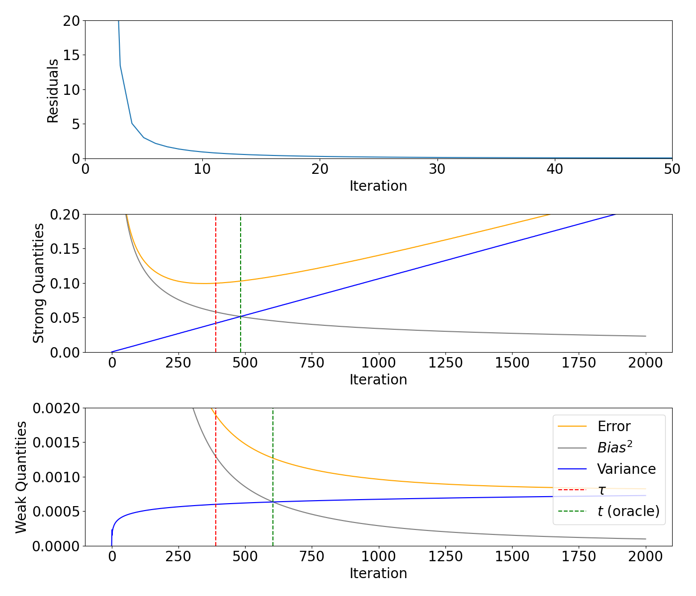
390
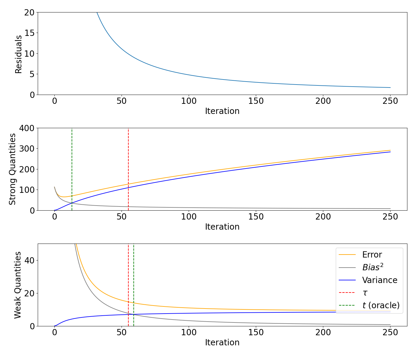
Bias/variance decomposition for a pertubated diagonal matrix#
Plot the residuals, weak and strong quantities.
D = 1000
normal_matrix = np.random.normal(0, 0.1, size=(D, D))
indices = np.arange(D) + 1
indices = np.arange(1, D + 1)
diagonal_values = 1 / np.sqrt(indices)
np.fill_diagonal(normal_matrix, diagonal_values)
design_matrix = normal_matrix

NOISE_LEVEL = 0.1
noise = np.random.normal(0, NOISE_LEVEL, D)
indices = np.arange(D) + 1
signal_supersmooth = 5 * np.exp(-0.1 * indices)
response = noise + design_matrix @ signal_supersmooth
max_iteration = 250

model_pertubation = es.Landweber(design_matrix, response, learning_rate = 0.01 , true_signal=signal_supersmooth, true_noise_level=NOISE_LEVEL)

model_pertubation.iterate(max_iteration)

# Stopping index
m_pertubation = model_pertubation.get_discrepancy_stop(D*(NOISE_LEVEL**2), max_iteration)

# Weak balanced oracle
weak_oracle_pertubation = model_pertubation.get_weak_balanced_oracle(max_iteration)

# Strong balanced oracle
strong_oracle_pertubation = model_pertubation.get_strong_balanced_oracle(max_iteration)


fig, axs = plt.subplots(3, 1, figsize=(14, 12))

axs[0].plot(range(0, max_iteration + 1), model_pertubation.residuals)
# axs[0].axvline(x=m, color="red", linestyle="--")
# axs[0].set_xlim([0, 50])
axs[0].set_ylim([0, 20])
axs[0].set_xlabel("Iteration")
axs[0].set_ylabel("Residuals")


axs[1].plot(range(0, max_iteration + 1), model_pertubation.strong_risk, color="orange", label="Error")
axs[1].plot(range(0, max_iteration + 1), model_pertubation.strong_bias2, label="$Bias^2$", color="grey")
axs[1].plot(range(0, max_iteration + 1), model_pertubation.strong_variance, label="Variance", color="blue")
axs[1].axvline(x=m_pertubation, color="red", linestyle="--")
axs[1].axvline(x=strong_oracle_pertubation, color="green", linestyle="--")
# axs[1].set_xlim([0, 50])
axs[1].set_ylim([0, 400])
axs[1].set_xlabel("Iteration")
axs[1].set_ylabel("Strong Quantities")

axs[2].plot(range(0, max_iteration + 1), model_pertubation.weak_risk, color="orange", label="Error")
axs[2].plot(range(0, max_iteration + 1), model_pertubation.weak_bias2, label="$Bias^2$", color="grey")
axs[2].plot(range(0, max_iteration + 1), model_pertubation.weak_variance, label="Variance", color="blue")
axs[2].axvline(x=m_pertubation, color="red", linestyle="--", label=r"$\tau$")
axs[2].axvline(x=weak_oracle_pertubation, color="green", linestyle="--", label="$t$ (oracle)")
# axs[2].set_xlim([0, 400])
axs[2].set_ylim([0, 50])
axs[2].set_xlabel("Iteration")
axs[2].set_ylabel("Weak Quantities")
axs[2].legend(loc = "upper right")

plt.tight_layout()

plt.show()
Total running time of the script: (0 minutes 54.372 seconds)