Note
Go to the end to download the full example code.
This is a comparison of Landweber and conjugate gradients#
import matplotlib.pyplot as plt
import numpy as np
import EarlyStopping as es
from scipy.sparse import dia_matrix
import timeit

np.random.seed(42)
plt.rcParams.update({"font.size": 20})
print("The seed is 42.")


import time
import numpy as np
import pandas as pd
from scipy.sparse import dia_matrix
import matplotlib.pyplot as plt
import seaborn as sns
import EarlyStopping as es

sns.set_theme(style="ticks")
np.random.seed(42)
The seed is 42.
Simulation Setting#
To make our results comparable, we use the same simulation setting as Blanchard et al. (2018) and Stankewitz (2020).
# Set parameters
sample_size = 1000
parameter_size = sample_size
max_iteration = sample_size
noise_level = 0.01
critical_value = sample_size * (noise_level**2)
# Create diagonal design matrices
indices = np.arange(sample_size) + 1
design = dia_matrix(np.diag(1 / (np.sqrt(indices))))
# Create signals
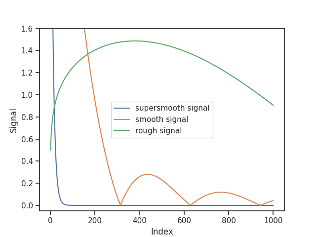
signal_supersmooth = 5 * np.exp(-0.1 * indices)
signal_smooth = 5000 * np.abs(np.sin(0.01 * indices)) * indices ** (-1.6)
signal_rough = 250 * np.abs(np.sin(0.002 * indices)) * indices ** (-0.8)
We plot the SVD coefficients of the three signals.
plt.plot(indices, signal_supersmooth, label="supersmooth signal")
plt.plot(indices, signal_smooth, label="smooth signal")
plt.plot(indices, signal_rough, label="rough signal")
plt.ylabel("Signal")
plt.xlabel("Index")
plt.ylim([-0.05, 1.6])
plt.legend()
plt.show()
Monte Carlo Study#
We simulate NUMBER_RUNS realisations of the Gaussian sequence space model.
# Specify number of Monte Carlo runs
NUMBER_RUNS = 10

# Set computation threshold
computation_threshold = 0

# Create observations for the three different signals
noise = np.random.normal(0, noise_level, (sample_size, NUMBER_RUNS))
observation_supersmooth = noise + (design @ signal_supersmooth)[:, None]
observation_smooth = noise + (design @ signal_smooth)[:, None]
observation_rough = noise + (design @ signal_rough)[:, None]
We create the models.
# Set interpolation boolean
interpolation_boolean = False

supersmooth_strong_empirical_error_cg = np.zeros(NUMBER_RUNS)
smooth_strong_empirical_error_cg = np.zeros(NUMBER_RUNS)
rough_strong_empirical_error_cg = np.zeros(NUMBER_RUNS)
supersmooth_weak_empirical_error_cg = np.zeros(NUMBER_RUNS)
smooth_weak_empirical_error_cg = np.zeros(NUMBER_RUNS)
rough_weak_empirical_error_cg = np.zeros(NUMBER_RUNS)

supersmooth_strong_empirical_error_landweber = np.zeros(NUMBER_RUNS)
smooth_strong_empirical_error_landweber = np.zeros(NUMBER_RUNS)
rough_strong_empirical_error_landweber = np.zeros(NUMBER_RUNS)
supersmooth_weak_empirical_error_landweber = np.zeros(NUMBER_RUNS)
smooth_weak_empirical_error_landweber = np.zeros(NUMBER_RUNS)
rough_weak_empirical_error_landweber = np.zeros(NUMBER_RUNS)

# Loop over the NUMBER_RUNS
for i in range(NUMBER_RUNS):
    # Create models for the supersmooth signal using Conjugate Gradients
    models_supersmooth_cg = es.ConjugateGradients(
        design,
        observation_supersmooth[:, i],
        true_signal=signal_supersmooth,
        true_noise_level=noise_level,
        interpolation=interpolation_boolean,
        computation_threshold=computation_threshold,
    )

    # Create models for the smooth signal using Conjugate Gradients
    models_smooth_cg = es.ConjugateGradients(
        design,
        observation_smooth[:, i],
        true_signal=signal_smooth,
        true_noise_level=noise_level,
        interpolation=interpolation_boolean,
        computation_threshold=computation_threshold,
    )

    # Create models for the rough signal using Conjugate Gradients
    models_rough_cg = es.ConjugateGradients(
        design,
        observation_rough[:, i],
        true_signal=signal_rough,
        true_noise_level=noise_level,
        interpolation=interpolation_boolean,
        computation_threshold=computation_threshold,
    )

    # Create models for the supersmooth signal using Landweber
    models_supersmooth_landweber = es.Landweber(
        design, observation_supersmooth[:, i], true_signal=signal_supersmooth, true_noise_level=noise_level
    )

    # Create models for the smooth signal using Landweber
    models_smooth_landweber = es.Landweber(
        design, observation_smooth[:, i], true_signal=signal_smooth, true_noise_level=noise_level
    )

    # Create models for the rough signal using Landweber
    models_rough_landweber = es.Landweber(
        design, observation_rough[:, i], true_signal=signal_rough, true_noise_level=noise_level
    )

    # Gather all estimates for the Conjugate Gradients models
    models_supersmooth_cg.gather_all(max_iteration)
    models_smooth_cg.gather_all(max_iteration)
    models_rough_cg.gather_all(max_iteration)

    # Iterate Landweber models for max_iter iterations
    models_supersmooth_landweber.iterate(max_iteration)
    models_smooth_landweber.iterate(max_iteration)
    models_rough_landweber.iterate(max_iteration)


    # Get the stopping index for the Landweber estimates
    supersmooth_stopping_index = models_supersmooth_landweber.get_discrepancy_stop(sample_size*(noise_level**2), max_iteration)
    smooth_stopping_index = models_smooth_landweber.get_discrepancy_stop(sample_size * (noise_level ** 2), max_iteration)
    rough_stopping_index = models_rough_landweber.get_discrepancy_stop(sample_size * (noise_level ** 2), max_iteration)


    # Calculate the strong empirical errors for Landweber estimates of the different signals
    supersmooth_strong_empirical_error_landweber[i] = models_supersmooth_landweber.strong_empirical_risk[supersmooth_stopping_index]
    smooth_strong_empirical_error_landweber[i] = models_smooth_landweber.strong_empirical_risk[smooth_stopping_index]
    rough_strong_empirical_error_landweber[i] = models_rough_landweber.strong_empirical_risk[rough_stopping_index]


    # Get the strong empirical errors for Conjugate Gradients estimates of the supersmooth signal
    supersmooth_strong_empirical_error_cg[i] = models_supersmooth_cg.strong_empirical_errors[
        models_supersmooth_cg.early_stopping_index
    ]

    # Get the strong empirical errors for Conjugate Gradients estimates of the smooth signal
    smooth_strong_empirical_error_cg[i] = models_smooth_cg.strong_empirical_errors[
        models_smooth_cg.early_stopping_index
    ]

    # Get the strong empirical errors for Conjugate Gradients estimates of the rough signal
    rough_strong_empirical_error_cg[i] = models_rough_cg.strong_empirical_errors[models_rough_cg.early_stopping_index]

    # WEAK EMPIRICAL ERRORS

    # Calculate the weak empirical errors for Landweber estimates of the different signals
    supersmooth_weak_empirical_error_landweber[i] = models_supersmooth_landweber.weak_empirical_risk[supersmooth_stopping_index]
    smooth_weak_empirical_error_landweber[i] = models_smooth_landweber.weak_empirical_risk[smooth_stopping_index]
    rough_weak_empirical_error_landweber[i] = models_rough_landweber.weak_empirical_risk[rough_stopping_index]

    # Get the weak empirical errors for Conjugate Gradients estimates of the supersmooth signal
    supersmooth_weak_empirical_error_cg[i] = models_supersmooth_cg.weak_empirical_errors[
        models_supersmooth_cg.early_stopping_index
    ]

    # Get the weak empirical errors for Conjugate Gradients estimates of the smooth signal
    smooth_weak_empirical_error_cg[i] = models_smooth_cg.weak_empirical_errors[models_smooth_cg.early_stopping_index]

    # Get the weak empirical errors for Conjugate Gradients estimates of the rough signal
    rough_weak_empirical_error_cg[i] = models_rough_cg.weak_empirical_errors[models_rough_cg.early_stopping_index]
/opt/hostedtoolcache/Python/3.12.7/x64/lib/python3.12/site-packages/EarlyStopping/landweber.py:115: UserWarning: No initial_value is given, using zero by default.
  warnings.warn("No initial_value is given, using zero by default.", category=UserWarning)
/opt/hostedtoolcache/Python/3.12.7/x64/lib/python3.12/site-packages/scipy/sparse/linalg/_dsolve/linsolve.py:603: SparseEfficiencyWarning: splu converted its input to CSC format
  return splu(A).solve
/opt/hostedtoolcache/Python/3.12.7/x64/lib/python3.12/site-packages/scipy/sparse/linalg/_matfuncs.py:76: SparseEfficiencyWarning: spsolve is more efficient when sparse b is in the CSC matrix format
  Ainv = spsolve(A, I)
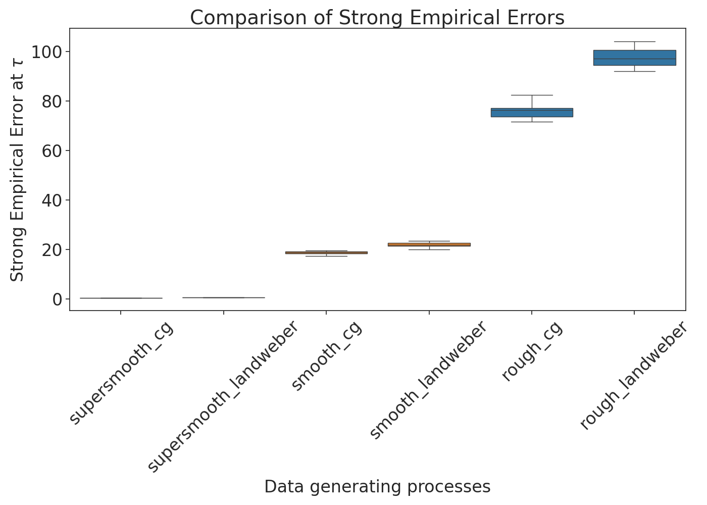
Strong Empirical Errors#
We plot the strong empirical errors of the conjugate gradient and Landweber estimates.
strong_empirical_errors_Monte_Carlo = pd.DataFrame(
    {
        # "algorithm": ["conjugate gradients"] * NUMBER_RUNS,
        "supersmooth_cg": supersmooth_strong_empirical_error_cg,
        "supersmooth_landweber": supersmooth_strong_empirical_error_landweber,
        "smooth_cg": smooth_strong_empirical_error_cg,
        "smooth_landweber": smooth_strong_empirical_error_landweber,
        "rough_cg": rough_strong_empirical_error_cg,
        "rough_landweber": rough_strong_empirical_error_landweber,
    }
)

strong_empirical_errors_Monte_Carlo = pd.melt(
    strong_empirical_errors_Monte_Carlo,
    # id_vars="algorithm",
    value_vars=[
        "supersmooth_cg",
        "supersmooth_landweber",
        "smooth_cg",
        "smooth_landweber",
        "rough_cg",
        "rough_landweber",
    ],
)

plt.figure(figsize=(14, 10))
strong_empirical_errors_boxplot = sns.boxplot(
    x="variable",
    y="value",
    data=strong_empirical_errors_Monte_Carlo,
    width=0.8,
    palette=["tab:purple", "tab:purple", "tab:orange", "tab:orange", "tab:blue", "tab:blue"],
)
strong_empirical_errors_boxplot.set_ylabel("Strong Empirical Error at $\\tau$", fontsize=24)  # Increase fontsize
strong_empirical_errors_boxplot.set_xlabel("Data generating processes", fontsize=24)  # Increase fontsize
strong_empirical_errors_boxplot.set_xticklabels(strong_empirical_errors_boxplot.get_xticklabels(), rotation=45)

strong_empirical_errors_boxplot.tick_params(axis="both", which="major", labelsize=24)  # Increase fontsize
plt.title("Comparison of Strong Empirical Errors", fontsize=28)  # Increase title fontsize
plt.tight_layout()
plt.show()
/home/runner/work/EarlyStopping/EarlyStopping/examples/plot_comparison.py:232: FutureWarning:

Passing `palette` without assigning `hue` is deprecated and will be removed in v0.14.0. Assign the `x` variable to `hue` and set `legend=False` for the same effect.

  strong_empirical_errors_boxplot = sns.boxplot(
/home/runner/work/EarlyStopping/EarlyStopping/examples/plot_comparison.py:241: UserWarning: set_ticklabels() should only be used with a fixed number of ticks, i.e. after set_ticks() or using a FixedLocator.
  strong_empirical_errors_boxplot.set_xticklabels(strong_empirical_errors_boxplot.get_xticklabels(), rotation=45)
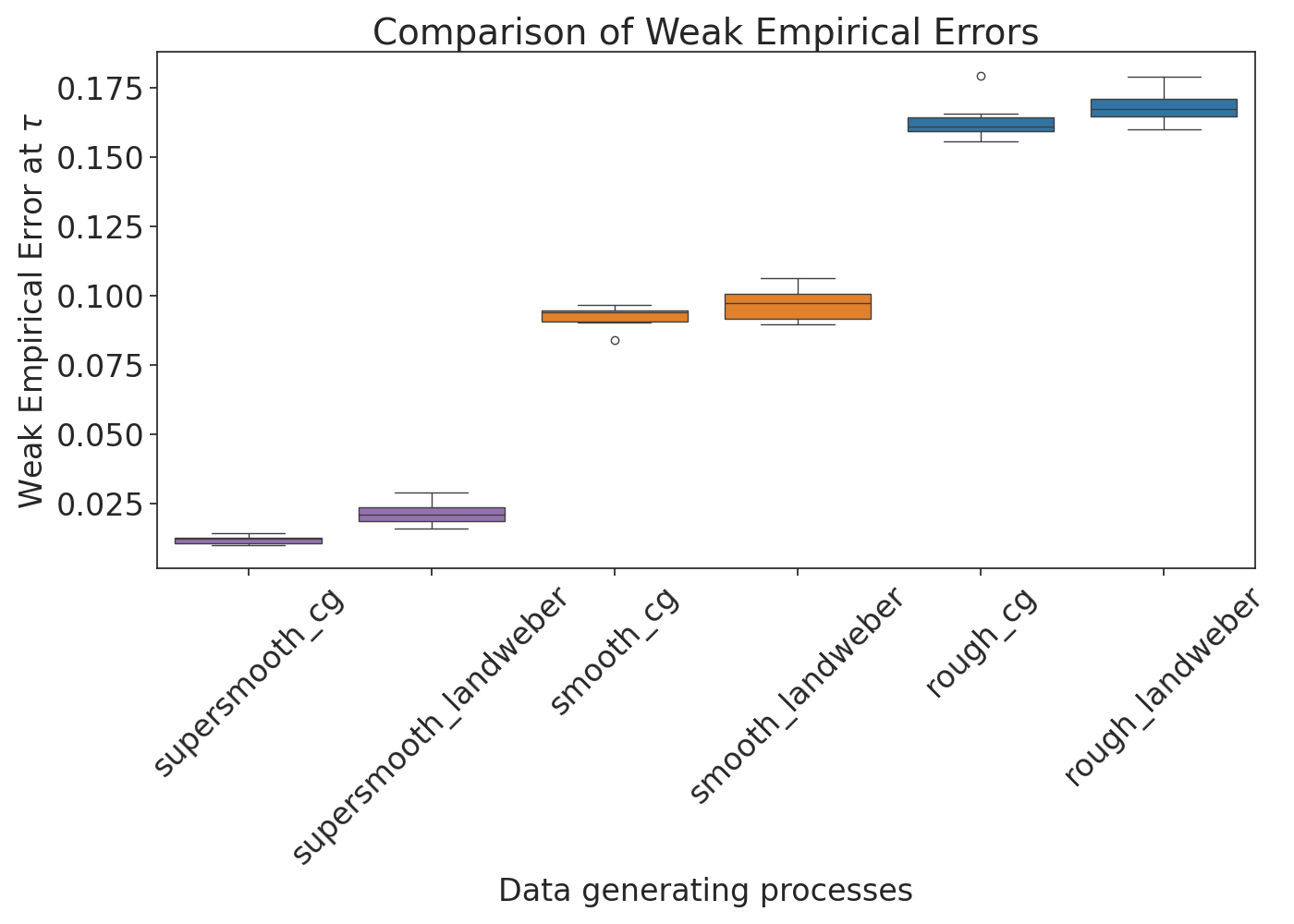
Weak Empirical Errors#
We plot the weak empirical errors of the conjugate gradient and Landweber estimates.
weak_empirical_errors_Monte_Carlo = pd.DataFrame(
    {
        # "algorithm": ["conjugate gradients"] * NUMBER_RUNS,
        "supersmooth_cg": supersmooth_weak_empirical_error_cg,
        "supersmooth_landweber": supersmooth_weak_empirical_error_landweber,
        "smooth_cg": smooth_weak_empirical_error_cg,
        "smooth_landweber": smooth_weak_empirical_error_landweber,
        "rough_cg": rough_weak_empirical_error_cg,
        "rough_landweber": rough_weak_empirical_error_landweber,
    }
)

weak_empirical_errors_Monte_Carlo = pd.melt(
    weak_empirical_errors_Monte_Carlo,
    # id_vars="algorithm",
    value_vars=[
        "supersmooth_cg",
        "supersmooth_landweber",
        "smooth_cg",
        "smooth_landweber",
        "rough_cg",
        "rough_landweber",
    ],
)

plt.figure(figsize=(14, 10))
weak_empirical_errors_boxplot = sns.boxplot(
    x="variable",
    y="value",
    data=weak_empirical_errors_Monte_Carlo,
    width=0.8,
    palette=["tab:purple", "tab:purple", "tab:orange", "tab:orange", "tab:blue", "tab:blue"],
)
weak_empirical_errors_boxplot.set_ylabel("Weak Empirical Error at $\\tau$", fontsize=24)  # Increase fontsize
weak_empirical_errors_boxplot.set_xlabel("Data generating processes", fontsize=24)  # Increase fontsize
weak_empirical_errors_boxplot.set_xticklabels(weak_empirical_errors_boxplot.get_xticklabels(), rotation=45)

weak_empirical_errors_boxplot.tick_params(axis="both", which="major", labelsize=24)  # Increase fontsize
plt.title("Comparison of Weak Empirical Errors", fontsize=28)  # Increase title fontsize
plt.tight_layout()
plt.show()
/home/runner/work/EarlyStopping/EarlyStopping/examples/plot_comparison.py:279: FutureWarning:

Passing `palette` without assigning `hue` is deprecated and will be removed in v0.14.0. Assign the `x` variable to `hue` and set `legend=False` for the same effect.

  weak_empirical_errors_boxplot = sns.boxplot(
/home/runner/work/EarlyStopping/EarlyStopping/examples/plot_comparison.py:288: UserWarning: set_ticklabels() should only be used with a fixed number of ticks, i.e. after set_ticks() or using a FixedLocator.
  weak_empirical_errors_boxplot.set_xticklabels(weak_empirical_errors_boxplot.get_xticklabels(), rotation=45)
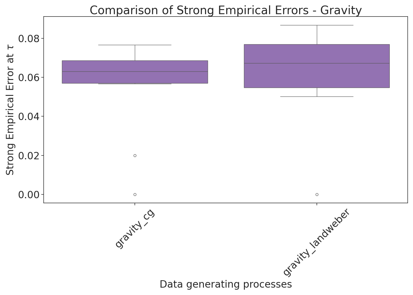
Montecarlo simmulation for the gravity example#
Gravity test problem from the regtools toolbox, see Hansen (2008) for details. Plot the residuals, weak and strong quantities.
sample_size_gravity = 100  # 2**9
a = 0
b = 1
d = 0.25  # Parameter controlling the ill-posedness: the larger, the more ill-posed, default in regtools: d = 0.25

t = (np.arange(1, sample_size_gravity + 1) - 0.5) / sample_size_gravity
s = ((np.arange(1, sample_size_gravity + 1) - 0.5) * (b - a)) / sample_size_gravity
T, S = np.meshgrid(t, s)

design_gravity = (
    (1 / sample_size_gravity)
    * d
    * (d**2 * np.ones((sample_size_gravity, sample_size_gravity)) + (S - T) ** 2) ** (-(3 / 2))
)
signal_gravity = np.sin(np.pi * t) + 0.5 * np.sin(2 * np.pi * t)
design_times_signal = design_gravity @ signal_gravity

# Set parameters
parameter_size = sample_size_gravity
max_iteration = 10000
noise_level = 10 ** (-2)

# Specify number of Monte Carlo runs
NUMBER_RUNS = 10

# Create observations
noise = np.random.normal(0, noise_level, (sample_size_gravity, NUMBER_RUNS))
observation_gravity = noise + design_times_signal[:, None]
We create the models.
gravity_strong_empirical_error_cg = np.zeros(NUMBER_RUNS)
gravity_weak_empirical_error_cg = np.zeros(NUMBER_RUNS)

gravity_strong_empirical_error_landweber = np.zeros(NUMBER_RUNS)
gravity_weak_empirical_error_landweber = np.zeros(NUMBER_RUNS)

count_landweber_fails = 0

for i in range(NUMBER_RUNS):
    # Create models for the gravity signal using Conjugate Gradients
    model_gravity_cg = es.ConjugateGradients(
        design_gravity,
        observation_gravity[:, i],
        true_signal=signal_gravity,
        true_noise_level=noise_level,
        interpolation=interpolation_boolean,
        computation_threshold=computation_threshold,
    )

    #  Create models for the gravity signal using Landweber
    model_gravity_landweber = es.Landweber(
        design_gravity,
        observation_gravity[:, i],
        true_signal=signal_gravity,
        learning_rate=1 / 30,
        true_noise_level=noise_level,
    )

    # Gather all estimates for the Conjugate Gradients models
    model_gravity_cg.gather_all(max_iteration)

    # Iterate Landweber models for max_iter iterations
    model_gravity_landweber.iterate(max_iteration)

    gravity_stopping_index = model_gravity_landweber.get_discrepancy_stop(sample_size_gravity * (noise_level ** 2), max_iteration)

    if gravity_stopping_index  == None:
        count_landweber_fails += 1
        continue

    # Get the strong empirical errors for Conjugate Gradients estimates of the gravity signal
    gravity_strong_empirical_error_cg[i] = model_gravity_cg.strong_empirical_errors[model_gravity_cg.early_stopping_index]
    gravity_weak_empirical_error_cg[i] = model_gravity_cg.weak_empirical_errors[model_gravity_cg.early_stopping_index]

    # Calculate the strong empirical errors for Landweber estimates of the gravity signal
    gravity_weak_empirical_error_landweber[i] = model_gravity_landweber.weak_empirical_risk[gravity_stopping_index]
    gravity_strong_empirical_error_landweber[i] = model_gravity_landweber.strong_empirical_risk[gravity_stopping_index]


print(f"Landweber failed {count_landweber_fails} attempts out of {NUMBER_RUNS}.")
/opt/hostedtoolcache/Python/3.12.7/x64/lib/python3.12/site-packages/EarlyStopping/landweber.py:115: UserWarning: No initial_value is given, using zero by default.
  warnings.warn("No initial_value is given, using zero by default.", category=UserWarning)
/opt/hostedtoolcache/Python/3.12.7/x64/lib/python3.12/site-packages/EarlyStopping/landweber.py:222: UserWarning: Early stopping index not found up to max_iteration. Returning None.
  warnings.warn("Early stopping index not found up to max_iteration. Returning None.", category=UserWarning)
Landweber failed 1 attempts out of 10.
Strong Empirical Errors Gravity#
We plot the strong empirical errors of the conjugate gradient and Landweber estimates.
strong_empirical_errors_Monte_Carlo = pd.DataFrame(
    {
        # "algorithm": ["conjugate gradients"] * NUMBER_RUNS,
        "gravity_cg": gravity_strong_empirical_error_cg,
        "gravity_landweber": gravity_strong_empirical_error_landweber,
    }
)

strong_empirical_errors_Monte_Carlo = pd.melt(
    strong_empirical_errors_Monte_Carlo,
    # id_vars="algorithm",
    value_vars=["gravity_cg", "gravity_landweber"],
)

plt.figure(figsize=(14, 10))
strong_empirical_errors_boxplot = sns.boxplot(
    x="variable",
    y="value",
    data=strong_empirical_errors_Monte_Carlo,
    width=0.8,
    palette=["tab:purple", "tab:purple"],
)
strong_empirical_errors_boxplot.set_ylabel("Strong Empirical Error at $\\tau$", fontsize=24)  # Increase fontsize
strong_empirical_errors_boxplot.set_xlabel("Data generating processes", fontsize=24)  # Increase fontsize
strong_empirical_errors_boxplot.set_xticklabels(strong_empirical_errors_boxplot.get_xticklabels(), rotation=45)

strong_empirical_errors_boxplot.tick_params(axis="both", which="major", labelsize=24)  # Increase fontsize
plt.title("Comparison of Strong Empirical Errors - Gravity", fontsize=28)  # Increase title fontsize
plt.tight_layout()
plt.show()
/home/runner/work/EarlyStopping/EarlyStopping/examples/plot_comparison.py:405: FutureWarning:

Passing `palette` without assigning `hue` is deprecated and will be removed in v0.14.0. Assign the `x` variable to `hue` and set `legend=False` for the same effect.

  strong_empirical_errors_boxplot = sns.boxplot(
/home/runner/work/EarlyStopping/EarlyStopping/examples/plot_comparison.py:414: UserWarning: set_ticklabels() should only be used with a fixed number of ticks, i.e. after set_ticks() or using a FixedLocator.
  strong_empirical_errors_boxplot.set_xticklabels(strong_empirical_errors_boxplot.get_xticklabels(), rotation=45)
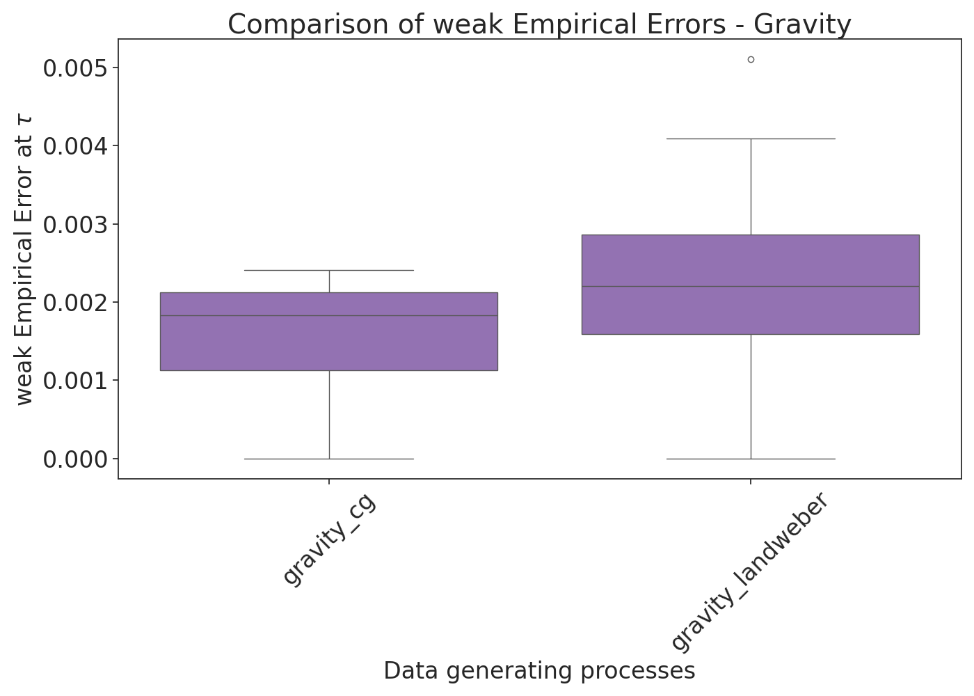
Weak Empirical Errors Gravity#
We plot the weak empirical errors of the conjugate gradient and Landweber estimates.
weak_empirical_errors_Monte_Carlo = pd.DataFrame(
    {
        # "algorithm": ["conjugate gradients"] * NUMBER_RUNS,
        "gravity_cg": gravity_weak_empirical_error_cg,
        "gravity_landweber": gravity_weak_empirical_error_landweber,
    }
)

weak_empirical_errors_Monte_Carlo = pd.melt(
    weak_empirical_errors_Monte_Carlo,
    # id_vars="algorithm",
    value_vars=["gravity_cg", "gravity_landweber"],
)

plt.figure(figsize=(14, 10))
weak_empirical_errors_boxplot = sns.boxplot(
    x="variable",
    y="value",
    data=weak_empirical_errors_Monte_Carlo,
    width=0.8,
    palette=["tab:purple", "tab:purple"],
)
weak_empirical_errors_boxplot.set_ylabel("weak Empirical Error at $\\tau$", fontsize=24)  # Increase fontsize
weak_empirical_errors_boxplot.set_xlabel("Data generating processes", fontsize=24)  # Increase fontsize
weak_empirical_errors_boxplot.set_xticklabels(weak_empirical_errors_boxplot.get_xticklabels(), rotation=45)

weak_empirical_errors_boxplot.tick_params(axis="both", which="major", labelsize=24)  # Increase fontsize
plt.title("Comparison of weak Empirical Errors - Gravity", fontsize=28)  # Increase title fontsize
plt.tight_layout()
plt.show()
/home/runner/work/EarlyStopping/EarlyStopping/examples/plot_comparison.py:441: FutureWarning:

Passing `palette` without assigning `hue` is deprecated and will be removed in v0.14.0. Assign the `x` variable to `hue` and set `legend=False` for the same effect.

  weak_empirical_errors_boxplot = sns.boxplot(
/home/runner/work/EarlyStopping/EarlyStopping/examples/plot_comparison.py:450: UserWarning: set_ticklabels() should only be used with a fixed number of ticks, i.e. after set_ticks() or using a FixedLocator.
  weak_empirical_errors_boxplot.set_xticklabels(weak_empirical_errors_boxplot.get_xticklabels(), rotation=45)
Total running time of the script: (2 minutes 36.218 seconds)